Visualising my Strava Network using R
by Niklas von Maltzahn
The recent release of the ggraph package for visualising networks in R got me interested in learning a little more about graph analysis and visualisation. My first thought was about what data I could use. I have a twitter account but twitter has been written about quite extensively so I searched for something different. Outside of my data-science interests I am a keen runner and use a website called Strava to manage my workouts. Strava allows you to connect with fellow athletes creating a perfect data set for my purposes.
Lucky for us, Strava provides a public API and there is an R package available on github at https://github.com/fawda123/rStrava.
The first thing to do is to register an app on the site and get hold of an app client id and app secret.
Prep
Lets start by loading some packages and connecting to the API:
#devtools::install_github('fawda123/rStrava') # install rStrava from github

# load packages
library(rStrava)
library(tidyverse)

# details you get after registering your app on strava.com
app_name <- 'Network Analysis'
app_client_id = ###
app_secret = '##########################'

# authenticate app and get an access token
stoken <- rStrava::strava_oauth(app_name = app_name,
                                app_client_id = app_client_id,
                                app_secret = app_secret,
                                cache=T)
Download the data
Once connected and authenticated we can access anything that is available on the api. Here is a link for further reading https://strava.github.io/api/.
First lets download a list of friends and list of followers.
# download my details
me <- get_athlete(stoken)

# get my friends from api
url <- 'https://www.strava.com/api/v3/athlete/friends'
my_friends <- get_pages(url_=url,
                       stoken=stoken,
                       All = T)

# extract my friend ids
my_friend_ids <- my_friends %>% map_chr('id')

saveRDS(my_friends,'my_friends.rds') # save for later use

# get my followers
url <- 'https://www.strava.com/api/v3/athlete/followers'
my_followers <- get_pages(url_=url,
                       stoken=stoken,
                       All = T)

saveRDS(my_followers,'my_followers.rds') # save for later use
And then a list of friend’s friends and friend’s followers:
# loop over each friend end download friends
friends_friends <- lapply(my_friends,function(friend) {
  id <- friend$id
  url <- sprintf('https://www.strava.com/api/v3/athletes/%s/friends',id)
  result <- get_pages(url_=url,
                               stoken=stoken,
                               All=T)
  return(result)
})
names(friends_friends) <- my_friend_ids
saveRDS(friends_friends,'friends_friends.rds') # save for later use

# loop over each friend end download followers
friends_followers <- lapply(my_friends,function(friend) {
  id <- friend$id
  url <- sprintf('https://www.strava.com/api/v3/athletes/%s/followers',id)
  result <- get_pages(url_=url,
                               stoken=stoken,
                               All=T)
  return(result)
})
names(friends_followers) <- my_friend_ids
saveRDS(friends_followers,'friends_followers.rds') # save for later use
The data is downloaded in JSON format that R has ingested as lists of lists. Each element has the following information:
my_friends[[1]] %>% names## [1] "id" "username" "resource_state" "firstname"
## [5] "lastname" "city" "state" "country"
## [9] "sex" "premium" "created_at" "updated_at"
## [13] "badge_type_id" "profile_medium" "profile" "friend"
## [17] "follower"Out interest is mainly in id but we can use the other fields to segment the network. Before we can do any analysis we will need to flatten/reshape this into a tidy data set.
Tidy the data
The strategy here is to flatten each list in to a row in a data frame. This works fairly well except for friends who don’t follow anyone. These are removed. A note on terminology: a follower follows a followee (very elegant).
# my_friends <- readRDS('my_friends.rds')
# my_followers <- readRDS('my_followers.rds')
# friends_friends <- readRDS('friends_friends.rds')
# friends_followers <- readRDS('friends_followers.rds')


# helper function that converts list to data frame
to_data_frame <- function(x) {
  # extract names
  names <- names(x)
  # loop over each element and remove if NULL
  for(y in names) {
    if (is.null(x[[y]])) {
      x[[y]] <- NULL
    }
  }
  # convert to data frame
  return(data.frame(x,stringsAsFactors = F))
}

# extract my friends as table
my_friends_table <- my_friends %>% map(~to_data_frame(.x)) %>% do.call('bind_rows',.)
my_friends_table$follower <- as.character(me$id)
my_friends_table$followee <- my_friends_table$id


# delete friends who have no friends
for (i in names(friends_friends)) {
  if (length(friends_friends[[i]])==0) {
    friends_friends[[i]] <- NULL
  }
}


# delete friends who have no followers
for (i in names(friends_followers)) {
  if (length(friends_followers[[i]])==0) {
    friends_followers[[i]] <- NULL
  }
}


# extract my friend's friends as a table
friends_friends_table <- map2(.x=names(friends_friends),.y=friends_friends,.f=function(x,y) {
  friends_table <- y %>% map(~to_data_frame(.x)) %>% do.call('bind_rows',.)
  friends_table$follower <- x
  friends_table$followee <- friends_table$id
  return(friends_table)
}) %>% do.call('bind_rows',.)


# extract my followers as a table
my_followers_table <- my_followers %>% map(~to_data_frame(.x)) %>% do.call('bind_rows',.)
my_followers_table$followee <- as.character(me$id)
my_followers_table$follower <- my_followers_table$id


# extract my friend's followers as a table
friends_followers_table <- map2(.x=names(friends_followers),.y=friends_followers,.f=function(x,y) {
  friends_table <- y %>% map(~to_data_frame(.x)) %>% do.call('bind_rows',.)
  friends_table$followee <- x
  friends_table$follower <- friends_table$id
  return(friends_table)
}) %>% do.call('bind_rows',.)


# convert ids
my_friends_table$followee <- as.integer(my_friends_table$followee)
my_friends_table$follower <- as.integer(my_friends_table$follower)


friends_friends_table$followee <- as.integer(friends_friends_table$followee)
friends_friends_table$follower <- as.integer(friends_friends_table$follower)


my_followers_table$followee <- as.integer(my_followers_table$followee)
my_followers_table$follower <- as.integer(my_followers_table$follower)


friends_followers_table$followee <- as.integer(friends_followers_table$followee)
friends_followers_table$follower <- as.integer(friends_followers_table$follower)

all_friends <- bind_rows(my_friends_table,friends_friends_table,my_followers_table,friends_followers_table)


# reorder for use with igraph
all_friends <- all_friends[,c('follower','followee',colnames(all_friends)[!colnames(all_friends) %in% c('follower','followee')])]
all_friends$my_friend <- all_friends$follower==me$id | all_friends$followee==me$id


saveRDS(all_friends,'all_friends.rds')
Finally we have all the information we need to create our network. Note how we re-ordered the all_friends data.frame so that the first two columns indicate each edge or relationship.
Create graph
Now let’s use igraph to create a graph object
# load igraph and ggraph packages
library(igraph)
library(ggraph)

# add direction flag for edges that lie on my id
all_friends$direction <- NA
all_friends$direction <- ifelse(all_friends$follower==me$id,'out',all_friends$direction)
all_friends$direction <- ifelse(all_friends$followee==me$id,'in',all_friends$direction)

# create graph from data frame
graph <- graph_from_data_frame(all_friends,directed = T)

# create flag for coloring my node differently to the rest
V(graph)$group <- ifelse(V(graph)$name==as.character(me$id),'me','others')

# create flag for whether someone is a friend, follower, both or neither
followers <- neighbors(graph,mode = 'in',v=as.character(me$id))$name
friends <- neighbors(graph,mode = 'out',v=as.character(me$id))$name
V(graph)$type <- case_when(
  V(graph)$name %in% as.character(me$id) ~ 'me',
  V(graph)$name %in% followers & V(graph)$name %in% friends ~ 'friend and follower',
  V(graph)$name %in% followers ~ 'follower',
  V(graph)$name %in% friends ~ 'friend'
)
Our graph data set contains 16,861 vertices and 23,537 edges. If we try to plot this, it will take a very long time. Let us rather focus on a subset of the graph called a neighourhood. Here we will subset the graph such that we only see my first order neighbours or friends/followers.
n <- neighborhood(graph,order=1,nodes=which(V(graph)$name %in% as.character(me$id)))
g1 <- subgraph(graph,v = unlist(n))
We now only have 102 nodes and 799 edges. Now we can plot with ggraph.
Plot Network
ggraph(g1,layout='nicely')+
  geom_edge_link()+
  geom_node_point()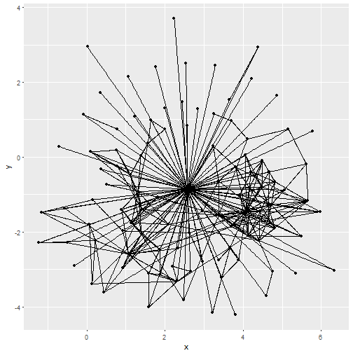
The plot shows each follower and followee in my network as a node or circle whilst the relationships are depicted by the edges or lines. We can clean this up a bit:
ggraph(g1,layout='nicely')+
  geom_edge_link(colour='gray',alpha=0.5)+ # make edges gray and transparent
  geom_node_point(aes(colour=group))+ # colour me differently to my neighbours
  scale_color_brewer(palette='Set1')+ # use a different colour palette
  theme_graph()+ # use the graph theme which is much neater
  labs(colour='') + # hide legend title
  theme(plot.title=element_text(hjust=0.5),legend.position = 'bottom') # center title and move legend to bottom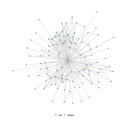
Then, let’s plot all edges with their directions as arrows:
ggraph(g1,layout='nicely')+
  geom_edge_fan(
    colour='gray',
    alpha=0.2,
    arrow = arrow(type = "closed", ends = "last",
                              length = unit(0.20, "cm"),
                              angle = 15)
  )+ # add arrows
  geom_node_point(aes(colour=group))+
  scale_color_brewer(palette='Set1')+
  theme_graph()+
  labs(colour='') +
  theme(plot.title=element_text(hjust=0.5),legend.position = 'bottom')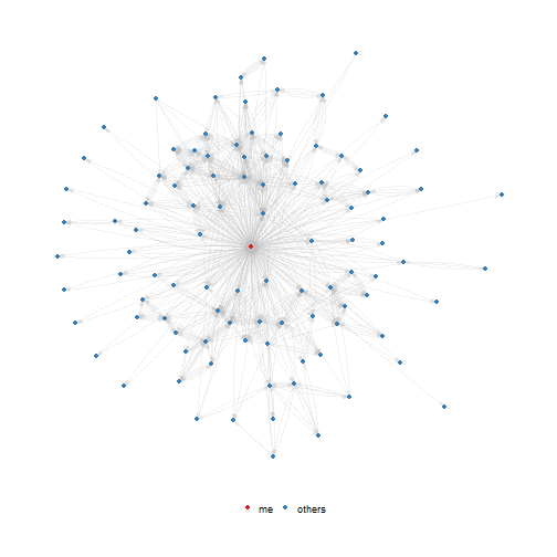
Finally, lets colour the nodes by type.
ggraph(g1,layout='nicely')+
  geom_edge_fan(
    colour='gray',
    alpha=0.2,
    arrow = arrow(type = "closed", ends = "last",
                              length = unit(0.20, "cm"),
                              angle = 15)
  )+ # add arrows
  geom_node_point(aes(colour=type))+
  scale_color_brewer(palette='Set1')+
  theme_graph()+
  labs(title='My Strava Network',colour='') +
  theme(plot.title=element_text(hjust=0.5),legend.position = 'bottom')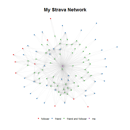
The chart shows that in most cases, my connections are both friend and follower however there are people that follow me that I don’t follow back. Similarly, I am following people that don’t follow me back.
ggraph is quite easy to use and fits in nicely with the existing tidyverse toolkit.
Next steps
In future, I would be interested in:
- expanding the size of the network
- identifying people with many friends/followers
- exploring graph metrics such as:
- degree
- pagerank
- creating an interactive plot using visNetwork
Thanks for reading!
Subscribe via RSS