Choosing where to buy a house in Cape Town, Southern Suburbs
by Niklas von Maltzahn
The Cape Town southern suburbs contain some of the Western Cape’s top schools but getting your child in to your desired school is very much dependent on living in the catchment area. These catchment areas are not always precisely defined with schools often just indicating that it should be the closest school to the child’s home.
My objective was to determine which areas would feed to a particular school based on distance.
We start by loading the ggmap package in order to geocode the set of schools.
# load some packages
library(ggmap)
suppressPackageStartupMessages(library(tidyverse))

# define candidate schools
school_names <- c('Rondebosch Boys Preparatory School',
                  'Groote Schuur Primary School, Rondebosch',
                  'Golden Grove Primary School, Rondebosch',
                  'Claremont Primary School, Claremont, Cape Town',
                  'Rosebank Junior School',
                  'Grove Primary School, Claremont, Cape Town'
                )
# geocode
coords <- geocode(school_names)
coords$name <- school_names
This gives a data frame:
| lon | lat | name |
|---|---|---|
| 18.47534 | -33.96447 | Rondebosch Boys Preparatory School |
| 18.47343 | -33.96927 | Groote Schuur Primary School, Rondebosch |
| 18.49046 | -33.97614 | Golden Grove Primary School, Rondebosch |
| 18.47072 | -33.97929 | Claremont Primary School, Claremont, Cape Town |
| 18.48917 | -33.96159 | Rosebank Junior School |
| 18.45988 | -33.98285 | Grove Primary School, Claremont, Cape Town |
We can now use ggmap to plot these on a map:
# load libraries for plotting
library(ggplot2)
library(ggrepel)

# clean names
coords <- coords %>% separate(name,into=c('clean_name','other'),sep = ',',remove = F)

# create bounding box for map and pad slightly bigger
lng_range <- diff(range(coords$lon))
lat_range <- diff(range(coords$lat))
margin <- 1

bbox <- c(
  left=min(coords$lon),
  bottom=min(coords$lat),
  right=max(coords$lon),
  top=max(coords$lat)
)
# add some padding
bbox <- bbox+c(-lng_range*margin,-lat_range*margin,lng_range*margin,lat_range*margin)

# download map from google
map <- get_map(location=bbox,zoom=14,color = 'bw')

# create a base map to work off of
p <- ggmap(map,
           extent = 'normal')+
  geom_point(data=coords,
             aes(x=lon,y=lat),col='darkblue',size=2)+
  coord_map(projection="mercator",
              xlim=c(attr(map, "bb")$ll.lon, attr(map, "bb")$ur.lon),
              ylim=c(attr(map, "bb")$ll.lat, attr(map, "bb")$ur.lat))+
  labs(x='',y='')+
  theme(axis.line = element_blank(),
        axis.text = element_blank(),
        axis.ticks = element_blank())

# plot schools
p+
  geom_text_repel(data=coords,
             aes(x=lon,y=lat,label=clean_name),col='darkblue')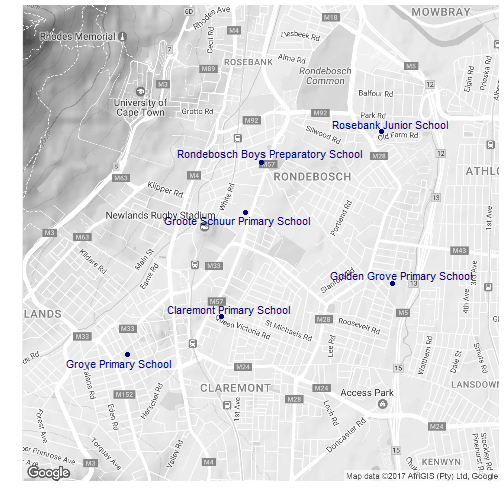
In order to separate the areas on the map in to catchment areas we need to define boundaries around each school that are equi-distant to neighbouring schools.
To do this lets define a grid across the map:
resolution <- 50 # set grid resolution

# generate a sequence across latitudes
lats <- seq(bbox[2],bbox[4],length=resolution)
# generate a sequence across longitudes
lngs <- seq(bbox[1],bbox[3],length=resolution)

# create all combinations
all <- expand.grid(lng=lngs,lat=lats)

# plot
p+
  geom_vline(xintercept = lngs,alpha=0.3,col='darkblue')+
  geom_hline(yintercept = lats,alpha=0.3,col='darkblue')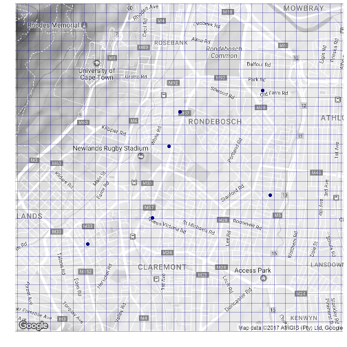
The aim will be to now map each grid point to its closest school which we can do using k nearest neighbours with k = 1. Note here that we pre-process the coordinates in to UTM (cartesian-type) coordinates for doing the distance calculation.
# load some spatial packages
suppressPackageStartupMessages(library(sp))
suppressPackageStartupMessages(library(rgdal))

# helper function to compute UTM coordinates for distance calculation
computeUTM <- function(df) {
  coordinates(df) <- c('lng','lat')
  proj4string(df) <- CRS("+proj=longlat +datum=WGS84")
  res <- spTransform(df, CRS(paste("+proj=utm +zone=",'34H'," ellps=WGS84",sep='')))
  return(as.data.frame(res))
}

# convert to UTM coordinates so that we can can calculate nearest schools
utm_all <- computeUTM(all[,c(1,2)])
utm_coords <- computeUTM(coords[,c('lon','lat')] %>% set_names(c('lng','lat')) )
utm_coords <- cbind(utm_coords,coords$clean_name)

library(class) # load class package for k nearest neighbours
closest_school <- class::knn1(utm_coords[,1:2],utm_all,utm_coords[,3])
all$school <- closest_school

# lets map again
p+
  geom_point(data=all,
             aes(x=lng,y=lat,col=school),size=2)+
  geom_point(data=coords,
             aes(x=lon,y=lat),size=3)+
  theme(legend.position = 'top')+
  labs(col='',caption='All points are mapped to their closest school')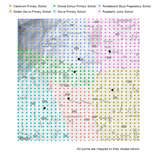
To get a more granular view let’s rerun the code segment with resolution set to 1000.
It would be nice to rather have a set of polygons define each region instead of a large set of points. It turns out that one can compute a convex hull which is the polygon that surrounds all the points.
Here is an example:
# generate two variables
x <- rnorm(100)
y <- rnorm(100)
df <- data.frame(x=x,y=y)

# compute convex hull
ch <- df %>%
    as.matrix %>%
    chull
# close polygon
ch <- c(ch,ch[1])

# plot
ggplot(df,aes(x,y))+
  geom_point()+
  geom_polygon(data=df[ch,],aes(x,y),col='red',fill=NA)+
  labs(title='Example of a convex hull')+
  theme_minimal()+
  theme(aspect.ratio=1)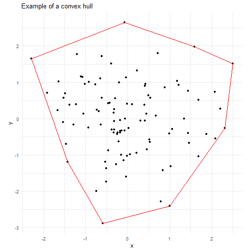
Now let’s apply this concept to our grid:
# create a helper function to compute the convex hull
compute_convexhull <- function(df) {
  ch <- df %>%
    select(lng,lat) %>%
    as.matrix %>%
    chull
  return(df[c(ch,ch[1]),])
}

# compute convex hull using grid
convex_hulls <- all %>%
  split(.$school) %>%
  map(~compute_convexhull(.)) %>%
  reduce(function(x,y) {
    union_all(x,y)
  })
The result looks like this:
| lng | lat | school |
|---|---|---|
| 18.48614 | -34.00188 | Claremont Primary School |
| 18.48660 | -34.00392 | Claremont Primary School |
| 18.48660 | -34.00412 | Claremont Primary School |
| 18.47622 | -34.00412 | Claremont Primary School |
| 18.47613 | -34.00392 | Claremont Primary School |
| 18.47595 | -34.00354 | Claremont Primary School |
| 18.47494 | -34.00143 | Claremont Primary School |
| 18.47246 | -33.99620 | Claremont Primary School |
| 18.46300 | -33.97621 | Claremont Primary School |
| 18.46116 | -33.97232 | Claremont Primary School |
This data frame should be enough to enclose our points in to a polygon.
Let’s plot the convex hulls as polygons on our map.
p+
  geom_polygon(data=convex_hulls,
               aes(x=lng,y=lat,group=school,fill=school),alpha=0.5)+
  geom_path(data=convex_hulls,
               aes(x=lng,y=lat,group=school,fill=school),alpha=0.5,col='white')+
  geom_point(data=coords,
             aes(x=lon,y=lat),col='darkblue',size=2)+
  labs(x='',y='',fill='',title='School Zones')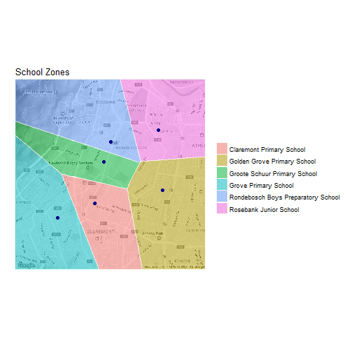
And there we have it! Now we know which areas one should buy a house in to maximise ones chance of getting in to a particular school.
Thanks for reading.
Subscribe via RSS